01 - Signals, Systems, and Sequences¶

Lecture 01 - 13 September 2021

The first lecture consists mostly of definitions and reminders. These are usually boring and rather cumbersome but are nevertheless needed.

Let’s start with our first definition: signals.

Signals¶

A signal is a MAP from time to some space:

\[\begin{align*} x\colon\ &\ t\longrightarrow y\\ &\mathcal{R}\mapsto\mathcal{R} \end{align*}\]

It is possible to restrict the domain and the codomain to \(\mathcal{Z} \subset \mathcal{R}\) so that we have four types of maps:

FROM \ TO	\(\mathcal{R}\)	\(\mathcal{Z}\)
\(\mathcal{R}\)	ANALOG	NOT USED
\(\mathcal{Z}\)	DIGITAL (theory)	DIGITAL (experiments)

SYSTEM¶

Similarly, systems are MAPs between signals

FROM \ TO	ANALOG	Digital
ANALOG	Analog System	Analog to Digital Converter (ADC)
DIGITAL	Digital to Analog converter (DAC)	Digital system; numeric system; processor

SEQUENCES¶

Sequences are maps from integer numbers to real or integer numbers:

\[\begin{align*} y\colon\ n&\longrightarrow y[n]\\ \mathcal{Z}&\longmapsto \mathcal{R} \textit{ or } \mathcal{Z} \end{align*}\]

Two remarkable sequences are the Delta / Impulse sequence and the Step Sequence.

Delta sequence¶

The delta sequency is defined in analogy to the diract delta and the Kronecker delta:

\[\begin{align*} \delta[n] = \delta_{n,0} = \left\{\begin{array}{lr} 1 \text{ if } n=0\\ 0 \text{ otherwise} \end{array}\right. \end{align*}\]

The analogy is straightforward:

\[\begin{align*} x(t) &= \int_{-\infty}^{+\infty} x(\tau) \delta (t-\tau) d\tau\\ x[n] &= \sum_{n_0 = -\infty}^{+\infty}x[x_0]\delta [n-n_0] \end{align*}\]

Step Sequence¶

Similarly, the step sequence is defined in analogy to the Heaviside theta:

\[\begin{align*} U[n] = \left\{\begin{array}{lr} 1 \text{ if } n\geq0\\ 0 \text{ otherwise} \end{array}\right. \end{align*}\]

import matplotlib.pyplot as plt
import numpy as np

t = np.arange(-5, 6, 1)
delta = np.zeros(t.shape); delta[ t.shape[0]//2] = 1
heavi = np.heaviside(t, 1)

fig, (ax1, ax2) = plt.subplots(1, 2, figsize=(15, 5))

ax1.title.set_text('Delta / Impulse Sequence')
ax1.scatter(t, delta, marker='o', label=r"$\delta[n]=\delta_{n,0}$")
ax1.set_xlabel('n'); ax1.set_ylabel('y[n]')
ax1.grid(True); ax1.legend(prop={'size': 14})
ax1.set_xticks(t)
ax1.set_ylim((-1, 2))

ax2.title.set_text('Step Sequence')
ax2.scatter(t, heavi, marker='o', label=r"$U[n]$")
ax2.set_xlabel('n'); ax2.set_ylabel('y[n]')
ax2.grid(True); ax2.legend(prop={'size': 14})
ax2.set_xticks(t)
ax2.set_ylim((-1, 2))

plt.show()
print("Left: Plot of the delta;\nRight: Plot of the step sequence.")

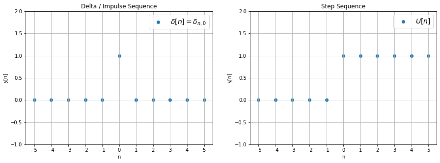
Left: Plot of the delta;
Right: Plot of the step sequence.

A sequence can be delayed or anticipated:

Delayed sequence: \(y[n] = x[n-n_0],\ n_0>0 \in \mathcal{Z}\);
Anticipated sequence: \(y[n] = x[n+n_0],\ n_0>0 \in \mathcal{Z}\).

These two operations are essential as they allow us to write all series as a sum of deltas with proper coefficients:

\[\begin{equation*} x[n] = \sum_{n_0 = -\infty}^{+\infty}x[n_0]\ \delta[n-n_0] = (x \ast \delta)[n] \end{equation*}\]

that is a discrete convolution between a sequence and a delta.

Periodic Sequences¶

A sequence \(x[n]\) is said to be periodic of period \(T\) if and only if (iff) \(x[n-T] = x[n]\ \forall n \in \mathcal{Z}\).

Energy¶

Finally, the energy of a system is defined as

\[\begin{equation*} \mathcal{E}(x[n]) = \sum_{n=-\infty}^{+\infty}\left| x[n] \right|^2 \end{equation*}\]

where the modulus was introduced to take care of signals \(\mathcal{Z}\rightarrow \mathcal{C}\).

Linear and Time-Invariant (LTI) Systems¶

As one can immagine, LTI systems are systems that are both linear and time invariant. Let’s consider a system:

\[\begin{align*} \mathcal{S}\colon\ \{x[n]\}&\longrightarrow \{y[n]\}\\ x[n]&\longmapsto y[n]=\mathcal{S}(x[n]) \end{align*}\]

Linear Systems¶

A system is linear iff given \(y_1[n]=\mathcal{S}(x_1[n])\) and \(y_2[n]=\mathcal{S}(x_2[n])\) the following relation holds:

\[\begin{equation*} \mathcal{S}(\alpha x_1[n] + \beta x_2[n]) = \alpha \mathcal{S}(x_1[n]) + \beta \mathcal{S}(x_2[n]) = \alpha y_1[n]+ \beta y_2[n] \end{equation*}\]

for every \(\alpha, \beta \in \mathcal{R}\).

Warning

Saying “a linear system is one for which the superposition principle holds” is a tautology because the superposition itself is defined via linearity.

One remarkable consequence of linearity is:

\[\begin{equation*} \mathcal{S}(x[n]) = \mathcal{S}\left(\sum_{k=-\infty}^{+\infty} x[k] \delta[n-k]\right) = \sum_{k=-\infty}^{+\infty} x[k] \mathcal{S}(\delta[n-k]) \end{equation*}\]

that is: a linear system is fully characterized by its impulse response \(h[n]=\mathcal{S}(\delta [n])\).

Time-Invariant Systems¶

A system is said to be time invariant iff

\[\begin{equation*} y[n] = \mathcal{S}(x[n]) \implies y_1[n] = \mathcal{x[n-n_0]} = y[n-n_0] \end{equation*}\]

that is: “to the same inputs correspond the same outputs without regard on when the input was sent”.

Notes of Advanced Electronics