07 - Bilinear Transform¶

Lecture 07 - 11 October 2021

Approximations for the simulation theorem¶

In the previous lecture, a way to approximate a system \(\tilde{G}(s)\) or \(\tilde{G}(\omega)\) with a discrete transfer function was seen. The result obtained is that \(V(z)\) is a perfect simulator for \(\tilde{G}(\omega)\) if and only if \(\tilde{G}(\omega)=V(z=e^{-i\omega T})\). It’s now time to search for a general way to obtain the discrete \(\tilde{V}(z)\) starting from the transfer function \(\tilde{G}(\omega)\). A first way would be to invert \(z=e^{-i\omega T}\rightarrow \omega=\frac{i}{T}ln(Z)\) but that would introduce a branch cut on \(\mathcal{R}_{0}^{-}\). A possibility is to abandon the search for an exact inversion and use a sufficiently close approximation \(\tilde{V} = \tilde{G}(\omega=f(z)) + \mathcal{o}\left( w^n\right)\).

Case 1: \(sin(\omega t)\)¶

Let’s start by writing \(sin(\omega t)\) as an exponential:

\[\begin{align*} sin(\omega t) = \frac{e^{i\omega t}-e^{-i\omega t}}{2i} = \frac{\frac{1}{z}-z}{2i} = \frac{1-z^2}{2iz} = \frac{1-z^2}{z}\frac{1}{2i} \end{align*}\]

And write the taylot series:

\[\begin{align*} sin(\omega t) = \omega t - \frac{(\omega T)^3}{6}+\mathcal{o}\left( (\omega T)^3 \right) \end{align*}\]

So that

\[\begin{align*} &\omega t - \frac{(\omega T)^3}{6}+\mathcal{o}\left( (\omega T)^3 \right) = \frac{1-z^2}{z}\frac{1}{2i}\\ \implies & \omega = \frac{z^2-1}{z}\frac{i}{2T}+\mathcal{o}\left( (\omega T)^3 \right)\\ \implies & \tilde{G}_{low pass}(\omega)=\frac{1}{1-i\omega \tau}=\frac{1}{1-i\tau \frac{1-z^2}{z}\frac{1}{2i}} = \frac{2Tz}{2Tz-\tau+\tau z^2} = \tilde{G}(z)=\tilde{V}(z) \end{align*}\]

Case 2: Bilinear Transform \(tan\left( \frac{\omega T}{2}\right)\)¶

\[\begin{align*} tan\left( \frac{\omega T}{2}\right) &= \frac{e^{i\omega T/2}- e^{-i\omega T/2}}{i\left( e^{i\omega T/2} + e^{i\omega T/2}\right)} = \frac{1}{i} \frac{1-e^{-i\omega T}}{1+e^{i\omega T}} = \frac{1}{i} \frac{z-1}{z+1} = \frac{\omega T}{2}+\mathcal{o}\left( (\omega T)^3 \right) \\ &\implies \omega \simeq \frac{2i}{T} \frac{z-1}{z+1} +\mathcal{o}\left( (\omega T)^3 \right) \end{align*}\]

Note: any function can be choosen to obtain the approximation but \(tan\left(\frac{\omega \pi}{2} \right)\) presents some nice features which will be discussed later.

Note 2: \(V(z)=\tilde{G}_{\mathcal{F}}\left(\omega=\frac{2i}{T} \frac{z-1}{z+1}\right) = \tilde{G}_{\mathcal{L}}\left(s=\frac{2}{T} \frac{z-1}{z+1}\right)\) is expected to be a good approximation of \(\tilde{G}_{\mathcal{F}}(\omega)=\tilde{G}_{\mathcal{L}}(s)\) if \(\omega T << 1\) i.e. if \(T_{SAMP}<< \frac{1}{\text{frequencies of interest}}\).

Bilinear transform and its properties¶

Let’s now see what happends when we apply a bilinear transform to a rational function:

\[\begin{align*} \tilde{G}(\omega)= \frac{N(\omega)}{D(\omega)} = \frac{\sum_{k=0}^Ma_k \omega^k}{\sum_{n=0}^N b_n \omega^n} \qquad \text{LTI} \end{align*}\]

Reality¶

Reality is conserved

\[\begin{align*} V(z)= \frac{\sum_{k=0}^Ma_k \left[ \frac{2i}{T} \frac{z-1}{z+1} \right]^k}{\sum_{n=0}^N b_n \left[\frac{2i}{T} \frac{z-1}{z+1} \right]^n} = \tilde{G}(\omega) \qquad V^*(z^*) = \frac{\sum_{k=0}^Ma_k \left[ \frac{2(-i)}{T} \frac{z-1}{z+1} \right]^k}{\sum_{n=0}^N b_n \left[\frac{2(-i)}{T} \frac{z-1}{z+1} \right]^n} = \tilde{G}(-\omega) \end{align*}\]

As we know that an analog system is real \(\iff\ \tilde{G}^*(\omega)=\tilde{G}(-\omega)\) we have proven the statement.

Causality¶

Causality can be proven but the proof is long and tedious. Just assume causality a priori or check the conditions \(0\not \in ROC; \infty \subset ROC\).

Bibo Stability¶

Reminder: An analog system is bibo stable \(\iff \mathcal{Re}\{poles\}<0\).
Reminder 2: A rational system can always be decomposed in a sum of fractions:

\[\begin{align*} \tilde{G}(s)&=\frac{N(s)}{D(s)}= ... + \frac{A}{(s-s_0)^n} \\ \xrightarrow[Transform]{Bilinear}& ... + \frac{A}{\left(\frac{2(-i)}{T} \frac{z-1}{z+1}-\frac{2(-i)}{T} \frac{z_0-1}{z_0+1}\right)^n} = ... + A\left[\frac{T}{2}\frac{(z+1)(z-1)}{z-z_0}\right]^N \end{align*}\]

and the poles stays of the same order after a bilinear transformation. It’s now possible to prove the preservation of bibo stability:

\[\begin{align*} s &= \frac{2}{T} \frac{z-1}{z+1} \rightarrow z=\frac{1+sT/2}{1-sT/2} = \frac{1+x+iy}{1-x-iy}\\ &\text{with }\frac{T}{2}s=x+iy,\quad x,y\in\mathcal{R}\\ &\implies \left| z_0 \right|^2 = 1+\frac{4x_0}{(x_0-1)^2+y_0^2} = 1+\frac{2T\mathcal{Re}\left\{s_0\right\}}{\left(1-\frac{T}{2}\mathcal{Re}\left\{s_0\right\} \right)^2 + \left(\mathcal{Im}\left\{s_0\right\} \right)^2} \end{align*}\]

by imposing \(\mathcal{Re}\{poles\}<0\) one obtains \(\left| z_0 \right|<1\), that is, all the poles \(\subset \Gamma_1\). As all the poles are strictly under \(\Gamma_1\) it is possible to find a curve that includes all the poles, is contained in \(\Gamma_1\), and encloses \(+\infty\). This implies that the system is Bibo stable. Another reason for which bilinear is preferred is that it is well-behaved near the boundaries of the Nyquist band:

Assume \(N>M\) (this can always be done by renaming eventual derivatives in the transfer function)

\[\begin{align*} \tilde{G}(\omega)&= \frac{N(\omega)}{D(\omega)} = \frac{\sum_{k=0}^Ma_k \omega^k}{\sum_{n=0}^N b_n \omega^n}\\ \implies \tilde{V}(z) &= \frac{\sum_{k=0}^Ma_k \left[ \frac{2i}{T} \frac{z-1}{z+1} \right]^k (z+1)^M}{\sum_{n=0}^N b_n \left[\frac{2i}{T} \frac{z-1}{z+1} \right]^n (z+1)^N} \frac{(z+1)^N}{(z+1)^M} = \frac{N'(z)}{D'(z)}(z+1)^{N-M} \end{align*}\]

The term \((z+1)^{N-M}\) is a leading term. Now let’s replace the simulation theorem:

\[\begin{align*} \tilde{G}(\omega)=V\left(z=e^{-i\omega T}\right) = \left. \frac{N'\left( z=e^{-i\omega T}\right)}{D'\left(z=e^{-i\omega T}\right)} \left( e^{-i\omega T}+1\right)^{N-M} \right|_{\omega = \pm \frac{\pi}{T} }=0 \end{align*}\]

That is, the tails of \(\tilde{x}(\omega)\) are smoothed out near the boundaries of the Nyquist band and ensure a nice transition to the cut region.

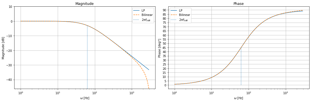
e.g. LOW PASS (actual implementation)¶

\[\begin{align*} \tilde{G}(\omega) &= \frac{1}{1-i\omega \tau} \\ V(z)&=\frac{1}{1-\frac{2\tau}{T}\frac{z-1}{z+1}} = \frac{z+1}{z\left(1+\frac{2\tau}{T}\right)-\left( \frac{2\tau}{T}-1\right)} \\ & =\frac{1-c}{2}\frac{z+1}{z-c} \qquad \text{with } c=\frac{1-T/2\tau}{1+T/2\tau} \\ V(z)&=\frac{Y(z)}{X(z)}= \frac{1-c}{2}\frac{z+1}{z-c} \implies y(z)\left( 1-\frac{c}{z}\right)=\frac{1-c}{2}\left( 1+\frac{1}{z}\right) x(z)\\ &\implies y[n]c-y[n-1]=\frac{1-c}{2}(x[n]+x[n-1]) \quad \text{Time domain} \end{align*}\]

Let’s now plot the Bode diagram for a low pass an for its bilinear transform. The two equations of interest are:

\[\begin{align*} \text{Ideal low pass} &\quad \tilde{G}(\omega)=\frac{1}{1-i\omega \tau}\\ \text{Discrete low pass} &\quad V\left(\omega\right)=\frac{1-c}{2}\frac{e^{-i\omega T}+1}{e^{-i\omega T}-c}\\ f_{3dB}&=10 \text{ Hz} \quad T = 2^{-10} \simeq 10^{-3} \end{align*}\]

import matplotlib.pyplot as plt
import numpy as np

##############
# PARAMETERS #
##############
T=1/1024 # Sampling time
omega = np.logspace(start=np.log10(1), stop=np.log10(0.9*np.pi/T), \
                    num=100, endpoint=True, base=10.0)
f3dB = 10 # Hz

omega0=2*np.pi*f3dB
tau = 1/(2*np.pi*f3dB)
#print("T=\t{:e}\ntau=\t{:e}".format(T, tau))

##################
# IDEAL LOW PASS #
##################
lp = 1/(1-1j*omega*tau) # Ideal Low pass 
mag_lp = 20*np.log10(np.abs(lp))
phase_lp = np.arctan(np.imag(lp)/np.real(lp))*180/np.pi

######################
# BILINEAR TRANSFORM #
######################
c = (1-T/(2*tau) ) / (1+T/(2*tau) )
lp_bt = 0.5*(1-c)*( np.exp(-1j*omega*T)+1 ) /(np.exp(-1j*omega*T)-c)
mag_lp_bt = 20*np.log10(np.abs(lp_bt))
phase_lp_bt = np.arctan( np.imag(lp_bt)/np.real(lp_bt))*180/np.pi

#########
# PLOTS #
#########
fig, ax = plt.subplots(1, 2, figsize=(15, 5))
ax[0].semilogx(omega, mag_lp, label="LP")    # Bode magnitude plot
ax[0].semilogx(omega, mag_lp_bt, "--", label="Bilinear")    # Bode magnitude plot

ax[1].semilogx(omega, phase_lp, label="LP")
ax[1].semilogx(omega, phase_lp_bt, "--", label="Bilinear")

ax[0].vlines(omega0, min(mag_lp_bt), 20*np.log10(np.abs(1/(1-1j))),linestyles=":", label=r"$2\pi f_{3dB}$")
ax[1].vlines(omega0, 0, 45, linestyles=":", label=r"$2\pi f_{3dB}$")

ax[0].set_title("Magnitude");  ax[1].set_title("Phase")
ax[0].set_xlabel(r"$\omega$ [Hz]"); ax[0].set_ylabel(r"Magnitude [dB]");
ax[1].set_xlabel(r"$\omega$ [Hz]"); ax[1].set_ylabel(r"Phase [deg°]");
ax[0].grid();   ax[1].grid()
ax[0].legend(); ax[1].legend()
ax[1].set_yticks([x for x in range(0, 91, 5)])
ax[0].set_ylim([min(mag_lp_bt), 10])

fig.tight_layout()
plt.show()

Notes of Advanced Electronics