06 - Simulation Theorem¶

Lecture 06 - 04 October 2021

Simulation of an analog system by means of a digital one¶

An interesting question is whether an analog system can be simulated by a digital one. The question is not as trivial as it sounds because a digital system deals only with discrete samples while an analog one has a continuou dynamic. A first intuition may be: “as Nyquist-Shannon allows to perfectly reconstruct a signal from its samples, all the information about the system must be contained in the samples and performing operations on them should be sufficient”. Formally. Given two system as shown in the following image:

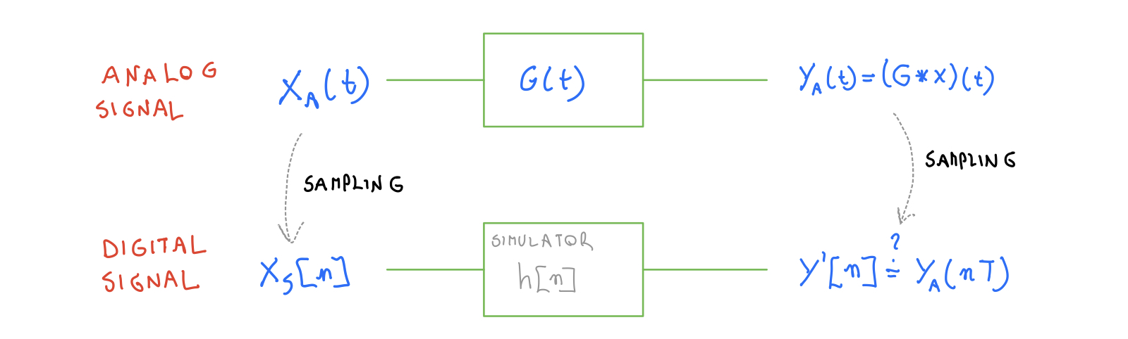
Simulation of an analog system by means of a digital one

does such \(h[n] : y'[n]=\sum_{k}h[n-k]x_s[k]\) exists? And, if so, how is it possible to find it? To answer this question let’s start with a function \(y'[n]=\sum_{k}h[n-k]x_s[k]\) and make some assumptions:

1a) Both \(x_A(t), G(t) \in \mathcal{L}^2\).¶

If this is true, it is possible to express the sampled output signal via its inverse Fuorier transform:

\[\begin{align*} y'[n]=\sum_k h[n-k]x_A(kT)= \sum_k h[n-k] \frac{1}{2\pi}\int_{-\infty}^{+\infty} \tilde{x}_A(\omega)e^{-i\omega k T} d\omega \end{align*}\]

2b) The simulator \(h[n]\) is BIBO Stable¶

If this is the case, it is possible to swap the summation and the integral in \(\sum_k \leftrightarrow \int_{-\infty}^{+\infty}\) without dealing with the convergence:

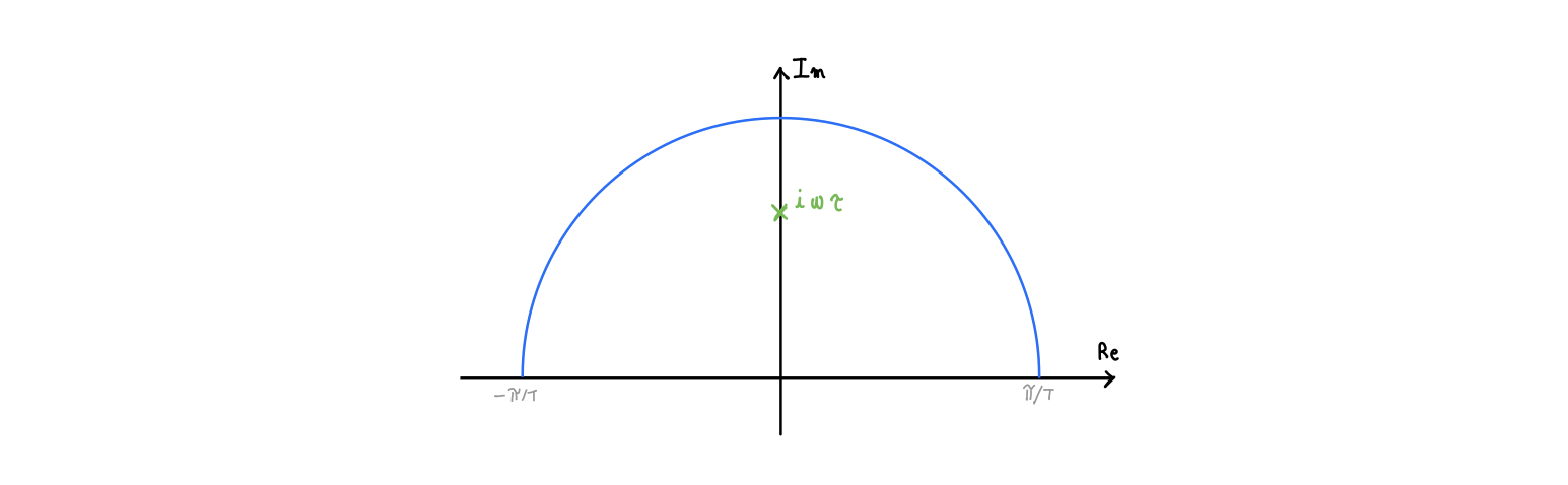
\[\begin{align*} y'[n] &= \frac{1}{2\pi}\int_{-\infty}^{+\infty} \tilde{x}_A(\omega) \sum_k h[n-k] e^{i\omega (n-k) T} e^{-i\omega n T} d\omega \qquad \text{define } z=e^{-i\omega T} \quad m=n-k\\ &= \frac{1}{2\pi}\int_{-\infty}^{+\infty} \sum_m h[m] z^{-m} e^{-i\omega n T} \tilde{x}_A(\omega) d\omega \\ &= \frac{1}{2\pi}\int_{-\infty}^{+\infty} H\left( z=e^{-i\omega Tn}\right) \tilde{x}_A(\omega) d\omega \end{align*}\]

where the condition \(z=e^{-i\omega T}\) was introduced to obtain the z-transform in conjunction with the condition \(z\in \Gamma_1 \subset ROC\) and the BIBO stability of the system.

Now, consider the sampling of the output signal \(y_A(t)\):

\[\begin{align*} \require{cancel} y_A[n]=y_A(nT)=\frac{1}{2\pi} \int_{-\infty}^{\infty} e^{-inT\omega} \cancelto{\tilde{y}(\omega)}{\tilde{G}(\omega)\tilde{x}(\omega)} d\omega \end{align*}\]

In order to satisfy the requirement \(y'[n]=y_A[n]\) we need:

\[\begin{align*} y'[n]-y_A[n]=0 \iff \frac{1}{2\pi} \int_{-\infty}^{\infty} e^{-inT\omega} \tilde{x}(\omega) \left[ H\left( z=e^{-i\omega Tn}\right) -\tilde{G}(\omega)\right] d\omega = 0 \end{align*}\]

The easiest solution to that equation is \(H\left( z=e^{-i\omega Tn}\right)=\tilde{G}(\omega)\) but it presents many problems, the most important of which is that it requires \(\tilde{G}(\omega)\) to be periodic with period T as \(H\left( z=e^{-i\omega Tn}\right)\) satisfies that property by default. A workaround is to force the whole integral to be zero with an assumption:

Assumption 2: The input signal \(\tilde{x}(\omega)\) is \(\frac{2\pi}{T}\) band limited¶

this forces the equality \(H\left( z=e^{-i\omega Tn}\right)=\tilde{G}(\omega)\) only on \(\left[-\frac{\pi}{T};\frac{\pi}{T} \right]\).

The discrete transfer function can be found by inverting the z-transform:

\[\begin{align*} h[n] &=\frac{1}{2\pi i} \oint_{\Gamma um 0\\ \Gamma\in ROC} H(z)z^{n-1}dz \qquad z=e^{-i\omega T} \iff \Gamma=\Gamma_1\\ &= -\frac{1}{2\pi i} \int_{-\frac{\pi}{T}}^{\frac{\pi}{T}} H(z=e^{-i\omega T})\left(e^{-i\omega T}\right)^{n-1} e^{-i\omega T} (-iT)d\omega\\ &= \frac{T}{2\pi} \int_{-\frac{\pi}{T}}^{\frac{\pi}{T}} e^{-i\omega nT}\tilde{G}(\omega) d\omega \end{align*}\]

Properties:¶

\(G(t)\in\mathcal{R} \iff h[n]\in\mathcal{R}\), proof by substitution.
BIBO STABILITY: must be checked on occurrence but it’s generally true
CAUSALITY IS NOT CONSERVED

Examples¶

First order low pass filter¶

\[\begin{align*} \require{mathtools} h[n]=\frac{T}{2\pi}\int_{-\frac{\pi}{T}}^{\frac{\pi}{T}}e^{-i\omega nT}\frac{1}{1-i\omega \tau} d\omega \xrightarrow[\text{Perfect sampling}]{T\rightarrow 0} \frac{T}{2\pi}\int_{-\infty}^{\infty}\frac{e^{-i\omega nT}}{1-i\omega \tau} d\omega = \frac{\theta(t)}{\tau}e^{-t/\tau} \end{align*}\]

but if \(T\not \rightarrow 0\) there is NO WAY to compute the integral. Not standard integral

The differentiator¶

The differentiator’s equation is \(\tau \frac{d}{dt}\rightarrow -i\omega\tau=\tilde{G}(\omega)\)

\[\begin{align*} \require{mathtools} h[n]&=\frac{T}{2\pi}\int_{-\frac{\pi}{T}}^{\frac{\pi}{T}}(-i\omega \tau)e^{-i\omega nT} d\omega \qquad x=\omega T\\ &= - \frac{i}{2\pi T}\int_{-\pi}^{\pi}e^{i nx} x dx = \left. \begin{cases} 0 \text{ if } n=0\\ \frac{(-1)^n}{nT} \text{ otherwise} \end{cases} \right\} = (-1)^n \frac{1-\delta[n]}{nT} \end{align*}\]

Backward interpretation of the simulation theorem¶

The one used above was the straightforward interpretation of the theorem. To overcome some of the problems it is possible to consider a backward intepretation of the simulation theorem, that is, the requirement are relaxed to \(y'[n]\simeq y[n]\) so that \(\tilde{G}(\omega)=H(z=e^{-i\omega T}) + o(\omega^n)\) in \(\left[ -\frac{\pi}{T}; \frac{\pi}{T} \right]\).

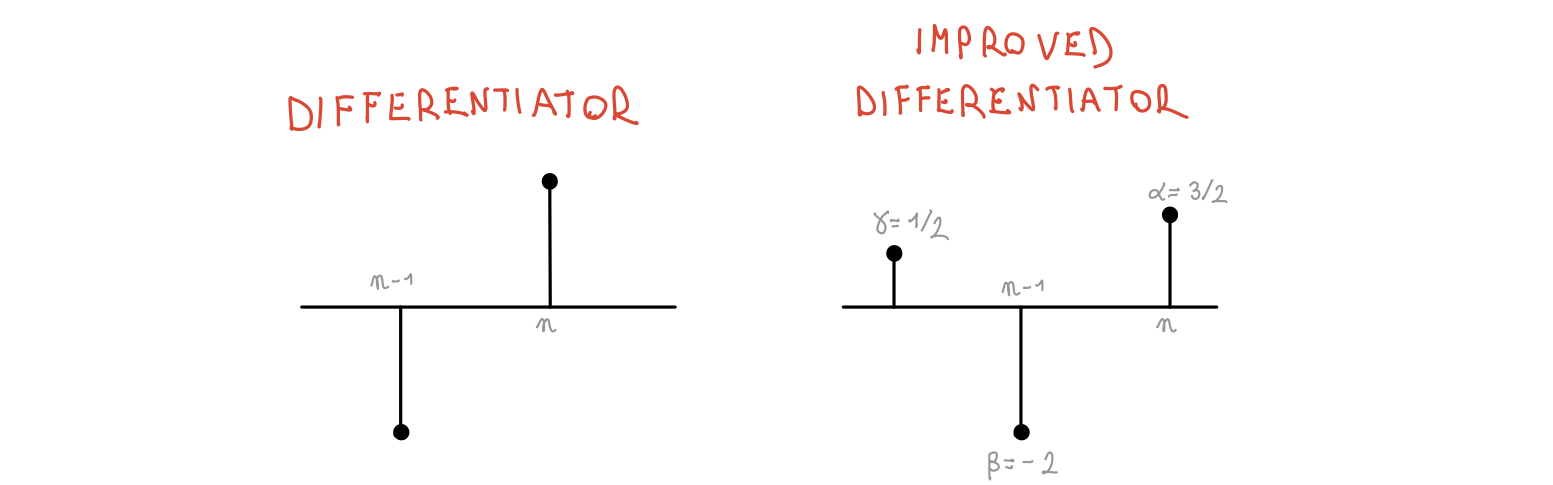
e.g. The differentiator (again)¶

Let’s take the approximate transfer function (which is given/found by an intuition): \(V[n]=\delta[n]-\delta[n-1]\) with z-transform \(V(z)=1 - \frac{1}{z}\). By taking the limit \(\omega T << 1\), it is possible to write:

\[\begin{align*} \tilde{G}(\omega)=V(z=e^{-i\omega T})=1-e^{i\omega T} \xrightarrow[]{\omega T \rightarrow0} -i\omega T + \mathcal{o}\left( (\omega T)^2 \right) \end{align*}\]

It is even possible to improve the accuracy by introducing new terms:

\[\begin{align*} V[n]&= \alpha \delta[n]+\beta \delta[n-1]+\gamma\delta[n-2] \implies V(z)=\alpha+\frac{\beta}{z}+\frac{\gamma}{z^2}\\ \tilde{V}(\omega)&=V(z=e^{-i\omega T}) = \alpha + \beta e^{i\omega T} + \gamma e^{2i\omega T} \\ &=\alpha+\beta+\gamma + (\beta+2\gamma)i\omega T + (\beta+4\gamma)(i\omega T)^2 + \mathcal{o}\left( (\omega T)^3 \right) \end{align*}\]

By comparing the approximated solution with the analitic one \(-i\omega T\) it is possible to write a system of equations and solve it:

\[\begin{align*} \begin{cases} \alpha+\beta+\gamma=0 \\ \beta+2\gamma=-1\\ \beta+4\gamma=0 \end{cases} \implies \begin{cases} \alpha = \frac{3}{2} \\ \beta =-2\\ \gamma=\frac{1}{2} \end{cases} \end{align*}\]

Notes of Advanced Electronics