03 - The Z-Transform¶

Lecture 03 - 20 September 2021

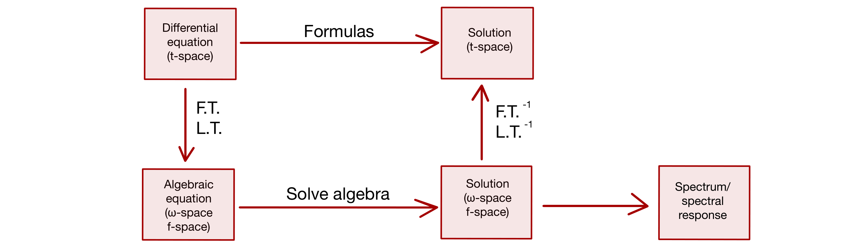
Equipped with the definitions and lemmas found in the last lecture it is possible to start talking about the z-transform. But first, it is necessary to draw some parallelisms with the solutions of a differential equation:

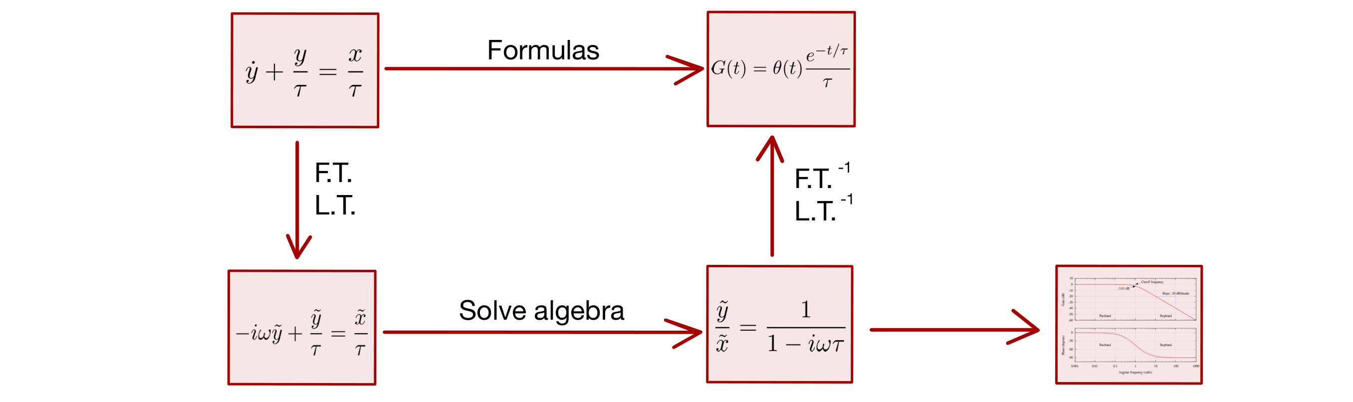
Solution of a differential equation with Fourier Transform / Laplace Transform

For example, with a low pass filter, the procedure becomes:
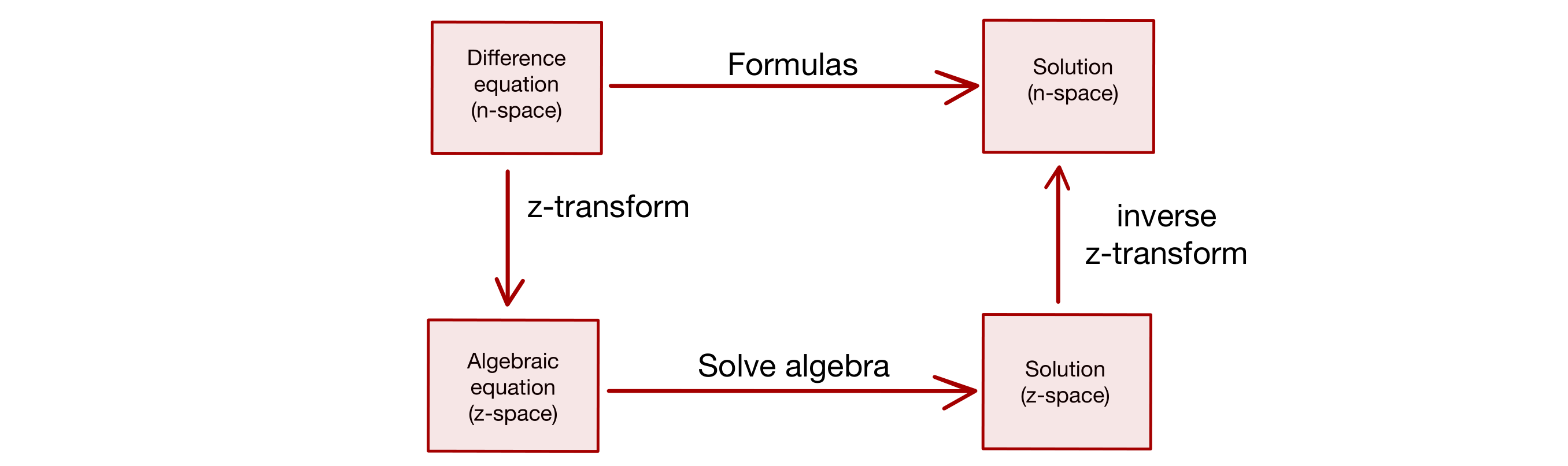
Solution of the low pass with Fourier Tranform

Similarly, a difference equation can be solved via an appropriate transform, the z-transform Solution of a difference equation with z-transform

The z-transform¶

Given a sequence \(x[n]\) we write the z-transform as

\[\begin{align*} Z\left(x[n]\right) = X(z) = \sum_{\forall n} z^{-n} x[n] \qquad \text{ with } \qquad z \in \textbf{R.O.C} \subseteq \mathcal{C}. \end{align*}\]

In the previous definition, R.O.C stands for Region Of Convergence, the region of the complex plane where the series converges to a finite value.

Some remarkable examples of z-transforms are:

Examples:¶

The delta¶

\[\begin{align*} Z\left(\delta[n]\right) = \sum_{n=-\infty}^{+\infty} z^{-n} \delta[n] = 1 \qquad \textbf{R.O.C} = \mathcal{C} \end{align*}\]

Step sequence¶

\[\begin{align*} Z\left(U[n]\right) &= \sum_{n=-\infty}^{+\infty} z^{-n} U[n] = \sum_{n=0}^{+\infty} z^{-n} = \frac{1}{1-1/z} = \frac{z}{z-1} \\ \text{ROC} &= \left\{ z : \frac{1}{|z|} < 1 \implies |z|>1\right\} \end{align*}\]

Step sequence (second case)¶

\[\begin{align*} Z\left(-U[-n-1]\right) &= -\sum_{n=-\infty}^{+\infty} z^{-n} U[-n-1] = - \sum_{n=1}^{+\infty} z^{n} = 1- \frac{1}{1-z} = \frac{z}{z-1} \\ \text{ROC} &= \left\{ z : \frac{1}{|z|} > 1 \implies |z|<1\right\} \end{align*}\]

It is possible to notice that two different functions led to the same z-transform but different R.O.C. A warning is due:

Warning

The z-transform is NOT sufficient to characterize a system in the z domain. The R.O.C. is part of the system too!

Properties of the z-transform¶

Let \(X[z] = Z(x[n])\).

Time shift¶

\[\begin{align*} Z\left(x[n-n_0]\right) = \sum_{n=-\infty}^{+\infty} z^{-n} x[n-n_0] = \sum_{n=-\infty}^{+\infty} z^{-(n-n_0)} z^{-n_0} x[n-n_0] = z^{-n_0} X(z) \end{align*}\]

Linearity¶

\[\begin{align*} Z\left(a x[n] + b y[n]\right) &= \sum_{n=-\infty}^{+\infty} z^{-n} (ax[n]+by[n]) = a X(z) + b X(z) \\ \text{ROC} &= \textbf{R.O.C}_x \cap \textbf{R.O.C}_y \end{align*}\]

Convolution¶

\[\begin{align*} Z\left(x[n]*y[n]\right) &= X(z) Y(z) \\ \text{ROC} &= \textbf{R.O.C}_x \cap \textbf{R.O.C}_y \end{align*}\]

There are two different proofs of this relation, one that exploits linearity and the time shift while the other is a more standard one that does not require any lemma. I’ll report both of them for completeness:

Standard proof¶

\[\begin{align*} Z\left(x[n]*y[n]\right) &= Z\left(\sum_k x[n-k]y[k] \right) = \sum_{n=-\infty}^{+\infty} \sum_{k=-\infty}^{+\infty} z^{-n} x[n-k] y[k] \\ &= \sum_{n=-\infty}^{+\infty} \sum_{k=-\infty}^{+\infty} z^{-(n-k)} z^{-k} x[n-k] y[k] = \sum_{k=-\infty}^{+\infty} \left( \sum_{n=-\infty}^{+\infty} z^{-(n-k)} x[n-k] \right) z^{-k} y[k] \\ &= \sum_{k=-\infty}^{+\infty} X(z) z^{-k} y[k] = X(z) Y(z) \\ \text{ROC} &= \textbf{R.O.C}_x \cap \textbf{R.O.C}_y \end{align*}\]

Proof via linearity¶

\[\begin{align*} Z\left(x[n]*y[n]\right) &= Z\left(\sum_k x[n-k]y[k] \right) = \sum_{k=-\infty}^{+\infty} Z(x[n-k])y[k] \\ &= \sum_{k=-\infty}^{+\infty} Z(x[n])z^{-k}y[k] = X(z) Y(z) \\ \text{ROC} &= \textbf{R.O.C}_x \cap \textbf{R.O.C}_y \end{align*}\]

Cascade of two systems¶

Cascade of two systems

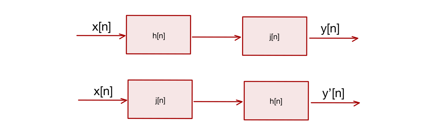
If the two systems are L.T.I. the two cascade are equivalent: \(y[n]=y'[n]\). The proof lies in the equality of the z-transform and the properties of the convolution. More than that, the two systems \(y[n]\) and \(y'[n]\) have the same R.O.C:

\[\begin{align*} y[n] &= h[n]*j[n] = Z^{-1}\left(h(z)j(z)\right) = Z^{-1}\left(j(z)h(z)\right) = j[n]*h[n] = y'[n] \\ \text{ROC} &= \text{ROC}_x \cap \text{ROC}_y \end{align*}\]

In the last properties, the notion of inverse z-transform was suggested. To give a formal definition of inverse z-transform some lemmas are needed.

Lemmas for inverse z-transform¶

Close path integral¶

The close path integral around (um) a single pole \(z_0\) depends only on the order of the pole:

\[\begin{align*} \frac{1}{2\pi i} \oint_{\Gamma\text{ um }z_0} (z-z_0)^n dz = \delta_{n, -1} \qquad \text{ with } n \in \mathcal{Z} \end{align*}\]

proof
Take a circle of radius \(r\) around \(z_0\) such that \(z=z_0+re^{i\phi}\). Then:

\[\begin{align*} \frac{1}{2\pi i} \oint_{\Gamma\text{ um }z_0} r^n e^{i\phi n} r e^{i\phi} i\ d\phi = \frac{r^{n+1}}{2\pi}\int_{0}^{2\pi} e^{i\phi (n+1)} d\phi = \begin{cases} 1 \qquad \text{if } n=-1\\ 0 \qquad \text{otherwise} \end{cases} \end{align*}\]

I like to call this lemma the “hidden logarithm lemma” because it reminds me of the integral \(\int x^n dx\). For every value of \(n\) the integral \(\int x^n dx\) remains a rational function, except when \(n=-1\). Similarly, when \(n\neq -1\) the function is an analytic function, which implies zero circuitation, while for \(n=-1\) a first-order pole is introduced.

Residual theorem¶

\[\begin{align*} \frac{1}{2\pi i} \oint_{\Gamma\text{ um }z_0} G(z) dz = \frac{1}{(n-1)!} \left[ \frac{d^{n-1}}{dz^{n-1}} G(z)(z-z_0)^n \right]_{z=z_0} \qquad \text{ with } n \in \mathcal{Z} \end{align*}\]

proof
Let’s consider a function \(H(z)=G(z)(z-z_0)^n\) which has NO POLES (\(\implies\) it is analytic). By writing its Laurent series one obtains:

\[\begin{align*} H(z)&=G(z)(z-z_0)^n = \sum_{k=0}^{+\infty} \frac{(z-z_0)^k}{k!} \left[ \frac{d^k}{dz^k} H(z)\right]_{z=z_0}\\ \implies& G(z) = \sum_{k=0}^{+\infty} \frac{(z-z_0)^{k-n}}{k!} \left[ \frac{d^k}{dz^k} H(z)\right]_{z=z_0} \end{align*}\]

By computing the integral using the previous lemma:

\[\begin{align*} \frac{1}{2\pi i} \oint_{\Gamma\text{ um }z_0} G(z) dz &= \sum_{k=0}^{\infty}\frac{1}{k!} \left[ \frac{d^k}{dz^k}H(z)\right]_{z=z_0}\cdot \frac{1}{2\pi i} \oint_{\Gamma\text{ um }z_0} (z-z_0)^n dz \\ &= \frac{1}{(n-1)!}\left[ \frac{d^{n-1}}{dz^{n-1}} G(z)(z-z_0)^n \right]_{z=z_0} \end{align*}\]

Inversion of the z-transform¶

If \(X(z)=Z(x[n])\) then \(x[n]=\frac{1}{2\pi i} \oint_{\Gamma\text{ um }z_0} X(z) z^{n-1} dz\)

proof

\[\begin{align*} \frac{1}{2\pi i} \oint_{\Gamma\text{ um } 0} X(z)z^{n-1} dz &= \frac{1}{2\pi i} \oint_{\Gamma\text{ um }0} \sum_{k}x[k]z^{-k}z^{n-1} dz \\ &= \frac{1}{2\pi i} \sum_{k} x[k] \oint_{\Gamma\text{ um } 0} z^{n-k-1} dz \\ &= \sum_{k}x[k] \delta_{n-k-1, -1} = x[n] \end{align*}\]

where the second equality assumes the R.O.C. allows swapping the summation and the integral.

Notes of Advanced Electronics