05 - Nyquist-Shannon Theorem¶

Lecture 05 - 27 September 2021

Sampling¶

Given a continuous function \(x_A(t)\), it is always possible to generate a discrete sequence by taking \(x[n]=x_A(nT)\), where \(T\) is the sampling time. A question should naturally arise: how good is it possible to reconstruct a signal \(x_{A}(t)\) from its sampled sequence? A first way to do that is to linearly interpolate between points:

import matplotlib.pyplot as plt
import numpy as np

x = np.linspace(0, 51, 10000)
ya= np.sin(x)*x**2 - np.cos(x)*np.log(x+0.1) + 3

n = np.linspace(0, 51, 30) # Change here the number of points
ys= np.sin(n)*n**2 - np.cos(n)*np.log(n+0.1) + 3


fig, ax = plt.subplots(1, 2, figsize=(15, 3))
ax[0].plot(x, ya, label="analog signal")
ax[0].plot(n, ys, lw=0, marker='.', color='r', label="sampling")

ax[1].plot(n, ys, marker='.', linestyle="--", mfc='r', mec='r', label="Linear reconstruction")

ax[0].set_xlim(0, 50); ax[1].set_xlim(0, 50);
ax[0].set_ylim(-2500, 2500); ax[1].set_ylim(-2500, 2500);
ax[0].grid(); ax[1].grid();
ax[0].legend(); ax[1].legend()

from IPython.display import display, Math, Latex
display(Math(r'f(x) = sin(x)x^2 - cos(x) log(x+0.1) + 3 \qquad \text{in }[0,51] \text{ with } T=1.7 \text{ (30 points)}'))

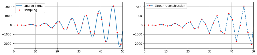
\[\displaystyle f(x) = sin(x)x^2 - cos(x) log(x+0.1) + 3 \qquad \text{in }[0,51] \text{ with } T=1.7 \text{ (30 points)}\]

but the results are not great. There exists an optimal way to reconstruct a function from the sampling, but it requires defining some quantities and making some rather general assumptions:

Definitions:¶

Sampling period/time: \(T\)
Sampling rate/frequency: \(f_s=T^{-1}\)
Nyquist frequency: \(F_{NY}= \frac{f_s}{2} \quad \omega_{NY} = 2\pi f_{NY} = \pi f_s = \frac{\pi}{T}\)
Nyquist band: \(f \in ]-f_{NY}; f_{NY}[ \quad \iff \quad f \in ]-\frac{\pi}{T}; \frac{\pi}{T}[\)

Assumptions¶

\(x_A(t)\) is \(\mathcal{L}^2\), that is, it has a Fourier Transform
\(x[n]=x_{A}(nT)\) is BIBO STABLE \(\implies \Gamma_1 \in \text{ROC}\left\{ x(z) \right\}\)

Let’s start by writing the sampled signal in terms of the Fourier transform of the analog signal:

\[\begin{align*} x_{s}[n] = x_A(nT) &= \frac{1}{2\pi}\int_{-\infty}^{+\infty} \tilde{x}_A(\omega)e^{-i\omega Tn} d\omega \\ &= \frac{1}{2\pi} \sum_{k=-\infty}^{+\infty} \int_{-\frac{\pi}{T}+\frac{2\pi}{T}k}^{\frac{\pi}{T}+\frac{2\pi}{T}k} \tilde{x}_A(\omega)e^{-i\omega Tn} d\omega \qquad \omega'=\omega-\frac{2\pi}{T}k\\ &= \frac{1}{2\pi} \sum_{k=-\infty}^{+\infty} \int_{-\frac{\pi}{T}}^{\frac{\pi}{T}} \tilde{x}_A\left(\omega'+\frac{2\pi}{T}k\right)e^{-i\left(\omega'+\frac{2\pi}{T}k\right) Tn} d\omega' \qquad e^{\frac{2\pi}{T}k Tn}=1 \\ &= \frac{1}{2\pi} \int_{-\frac{\pi}{T}}^{\frac{\pi}{T}} \sum_{k=-\infty}^{+\infty} \tilde{x}_A\left(\omega'+\frac{2\pi}{T}k\right)e^{-i\omega' Tn} d\omega' \end{align*}\]

At the same time, the sequence \(x_s[n]\) can be expressed via the inverse z-transform around \(\Gamma_1\) clockwise:

Circonference Gamma 1 travelled clockwise

\[\begin{align*} x_{s}[n] &= \frac{1}{2\pi i} \oint_{\Gamma \in ROC} x_s(z) z^{n-1} \qquad z=e^{-i\omega t} \qquad dz=(-iT)e^{-i\omega T}\\ &= - \frac{1}{2\pi i} \oint_{-\frac{\pi}{T}}^{\frac{\pi}{T}} x_s(e^{-i\omega t}) e^{-i\omega T (n-1)} (-iT) e^{-i\omega t} d\omega \\ &= \frac{T}{2\pi} \oint_{-\frac{\pi}{T}}^{\frac{\pi}{T}} x_s(e^{-i\omega t}) e^{-i\omega n T} d\omega\\ \end{align*}\]

By composing this expression with the one obtained above it is possible to obtain:

Nyquist-Shannon precursor theorem

\(T x_s\left(z=e^{-i\omega T}\right) = \sum_{k} \tilde{x}_A\left( \omega+\frac{2\pi}{T}k\right)\) with \(\omega\in \left] -\frac{\pi}{T}; \frac{\pi}{T}\right[\)

WARNING: The function on the right must be periodic with period \(\frac{2\pi}{T}\) due to the nature of the complex exponential. In contrast, the function on the left wasn’t assumed to be periodic so the expression can’t be true in general. To circumvent this issue, we make a third assumption:

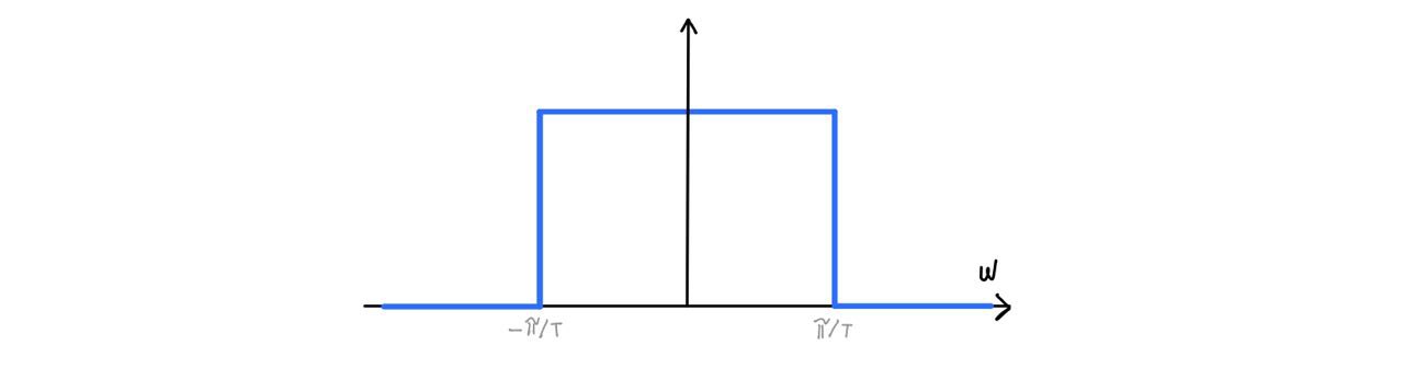
Assume \(x_A(t)\) to be band limited on \(\left] -\frac{\pi}{T}; \frac{\pi}{T}\right[\), that is \(\tilde{x}_A(\omega)=0 \text{ if } \left| \omega\right| \geq \frac{\pi}{T}\).

This assumption allows us to unwrap the summation and force the equality in the precursor theorem:

\[\begin{align*} \require{cancel} T x_s\left(z=e^{-i\omega T}\right) =\tilde{x}_A\left( \omega\right) + \cancelto{0}{ \tilde{x}_A\left( \omega+\frac{2\pi}{T}\right) } +\ ... \end{align*}\]

It is now time to go back to the time domain:

\[\begin{align*} \require{color} x_A(t) &= \frac{1}{2\pi}\int_{-\infty}^{+\infty} \tilde{x}_A(\omega)e^{-i\omega T} d\omega \qquad \text{exploit hypothesis 3.}\\ &= \frac{1}{2\pi}\int_{-\frac{\pi}{T}}^{+\frac{\pi}{T}} \tilde{x}_A(\omega)e^{-i\omega T} d\omega \qquad \text{use the precursor theorem}\\ &= \frac{1}{2\pi}\int_{-\frac{\pi}{T}}^{+\frac{\pi}{T}} T x_s(z=e^{-i\omega T}) e^{-i\omega T} d\omega = \frac{T}{2\pi}\int_{-\frac{\pi}{T}}^{+\frac{\pi}{T}} \sum_{n} x_s[n]e^{i\omega n T -i\omega t} d\omega \\ &= \frac{T}{2\pi}\sum_{n} x_s[n] \int_{-\frac{\pi}{T}}^{+\frac{\pi}{T}} e^{i\omega n T -i\omega t} d\omega = \frac{T}{2\pi}\sum_{n} x_s[n] \int_{-\frac{\pi}{T}}^{+\frac{\pi}{T}} e^{i\omega (n T-t)} d\omega \\ &= \frac{T}{2\pi}\sum_{n} x_s[n] \left[ \frac{e^{i\omega(nT-t)}}{i(nT-t)} \right]^{\frac{\pi}{T}}_{-\frac{\pi}{T}} = \cancel{\frac{T}{2\pi}} \sum_{n} x_s[n] \frac{e^{i(nT-t)\frac{\pi}{T}}+e^{-i(nT-t)\frac{\pi}{T}}}{i(nT-t) \textcolor[rgb]{0.75,0.75,0.75}{\frac{2\pi}{T}} } \\ &= \sum_{n} x_s[n] sinc\left[ (nT-t)\frac{\pi}{T}\right]\\ \end{align*}\]

Nyquist-Shannon theorem in the time domain

\(x_A(t)=\sum_{n} x_s[n] sinc\left[ (nT-t)\frac{\pi}{T}\right]\)

The condition \(\tilde{x}_A(\omega)=0\) if \(\left|\omega\right|\geq \frac{\pi}{T}\) or \(\left|f\right|\geq \frac{1}{2T}=f_{NY} \implies \max_f\left\{ \left|f\right|\right\}<\frac{1}{2T}=f_{NY}\).

Aliasing¶

Let’s now analyze what happens in the case of undersampling, that is, if \(f_S < f_{NY}\).

definitions¶

Reconstructed Signal: \(x_R(t)=\sum_{n} x_s[n] sinc\left[ (nT-t)\frac{\pi}{T}\right]\) with \(x_s[n]=x_A(nT)\)
Folding: \(x_F(\omega)=\sum_{n}\tilde{x}_A\left( \omega+\frac{2\pi}{T}k \right) \implies \tilde{x}_F(\omega)=T X_s(z=e^{-i\omega T})\)
Window on Nyquist band: \(W(\omega)=\theta\left(\omega+\frac{\pi}{T}\right)-\theta\left(\omega-\frac{\pi}{T}\right)\)
Alias: \(\tilde{x}_{alias}(\omega)=W(\omega)\tilde{x}_F(\omega)\).

Properties of the alias function:

It is \(\pi/T\) band limited due to \(W(\omega)\)
\(\sum_n \tilde{x}_{alias}\left( \omega+\frac{2\pi}{T}k \right) = \sum_n \tilde{x}_{F}\left( \omega+\frac{2\pi}{T}k \right)W\left( \omega+\frac{2\pi}{T}k \right) = \tilde{x}_{F}\left( \omega\right)\cancelto{1}{\sum_nW\left( \omega+\frac{2\pi}{T}k \right)} \\ \implies \tilde{x}_{F}\left( \omega\right) = \sum_n \tilde{x}_{alias}\left( \omega+\frac{2\pi}{T}k \right) \)
If \(\omega \in \left] -\frac{\pi}{T};\frac{\pi}{T} \right[\) \(\implies\) \(\tilde{x}_{alias}(\omega)=\tilde{x}_{F}(\omega) = T x_s\left( z=e^{-i\omega T} \right)\) \(\implies\) \(\mathcal{FT}^{-1}\left\{ \tilde{x}_{aliasing}(\omega) \right\} = x_R(t)= \sum_{n} x[n]sinc\left[ (t-nT)\frac{\pi}{T}\right]\)

By assuming that \(\tilde{x}_{alias}(\omega)\) is band limited it is possible to obtain \(\tilde{x}_{alias}(\omega)=\tilde{x}_{A}(\omega) \implies x_R(t)=x_A(t)\). On the other hand, if \(\tilde{x}_{alias}(\omega)\) is NOT band limited the reconstruction is not possible: Comparision between an unersampled signal and a properly samped one

Warning

DO NOT validate the goodness of a reconstruction on the sampled points as they are always reconstructed perfectly: \(\lim_{t\rightarrow nT}sinc\left[(t-nT)\frac{\pi}{T}\right]=1 \implies x_R(t=nT)=x[n]\ \forall n\)

Exercise¶

Take \(\mathcal{Re}\left\{e^{i\omega_0 t}\right\} = cos(\omega_0 t)\) with \(\omega_0=2\pi f_0\) and sample it first with \(T<\frac{1}{2f_0}\) and then with \(T>\frac{1}{2f_0}\). Reconstruct the two signals and check the differences.

Notes of Advanced Electronics