02 - Stability of Systems and Difference Equations¶

Lecture 02 - 14 September 2021

In the previous lecture, we gave some basic definitions and showed that an LTI system is fully characterized by its impulse response.

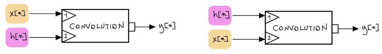
An interesting property of LTI systems is that it is possible to imagine the impulse response and the input sequence as the two inputs of a convolution. This means that it is possible to freely swap the input sequence and the impulse response.

\[\begin{align*} x[n] \rightarrow [SYSTEM] \rightarrow y[n] &\implies (x[n], h[n]) \rightarrow [CONVOLUTION] \rightarrow y[n] \\ &\implies (h[n], x[n]) \rightarrow [CONVOLUTION] \rightarrow y[n] \end{align*}\]

Matematically:

\[\begin{align*} y[n] = \sum_{k=-\infty}^{\infty} x[n] h[n-k]\quad \xrightarrow[k'=n-k]{k=k'-n} \quad \sum_{k'=-\infty}^{\infty} x[n-k'] h[k'] \end{align*}\]

We will now discuss three important features that a system can have, namely reality, causality / non-causality, and marginal stability / Bibo stability.

Key properties of a system¶

Reality¶

A system is said to be real iff \(h[n]\in \mathcal{R}\).

(Non) Causality¶

A system is said to be causal (or nonanticipative) iff \(h[n] = 0 \textit{ if } n<0\). An equivalent definition is: the output \(y[n_{0}]\) depends on only the input \(x[n]\) for values of \(n < n_{0}\). The idea behind this property is that the output depends only on past inputs and not on future inputs.

A non-causal system is defined by substituting the “less than” with a “greater than”:
A system is said to be causal (or nonanticipative) iff \(h[n] = 0 \textit{ if } n>0\). An equivalent definition is: the output \(y[t_{0}]\) depends on only the input \(x[n]\) for values of \(n>n_{0}\).

Note

A system can be BOTH causal and NON CAUSAL. A class of systems that satisfy this properties are amplifiers \(h[n]= \alpha\ \delta[n]\). These kind of systems respect both conditions as they have \(h[n]=0\) for both \(t<0\) and \(t>0\).

An intuitive way to remember causality is the following: consider a causal linear system defined as:

\[\begin{equation*} y[n] = \sum_{k=-\infty}^{+\infty} x[k] h[n-k] \end{equation*}\]

and label the current time step as zero \(n=0\):

\[\begin{equation*} y[0] = \sum_{k=-\infty}^{+\infty} x[k] h[-k] \end{equation*}\]

The usual definition of cauality implies that the system can not depend on future inputs because we don’t know those inputs yet. Future inputs are labelled with positive indices, e.g. \(x[1], x[2], etc\). For those values of \(k\) we have \(h[-1], h[-2], etc\). So, the only way for the system to remove the dependence on future inputs is to have \(h[l] = 0 \iff l<0\).

Marginal Stability¶

A system is marginal stable iff \(\exists L<+\infty\ :\ |h[n]| \leq L\ \forall n\).

An example of marginal stable system is one with \(h[n]=U[n]= 1\) (the integrator):

\[\begin{equation*} y[n] = \sum_{k=-\infty}^{+\infty} x[k]\ U[n-k] = \sum_{k=-\infty}^{n} x[k] \end{equation*}\]

BIBO Stability¶

A system is BIBO Stable (Bounded Input - Bounded Output) if to each and every bounded input \(x[n]\) it corresponds a bounded output.

\[\begin{equation*} \forall\ x[n]\ :\ |x[n]|<+\infty \implies \exists L<\infty\ :\ |y[n]|<L\quad \forall n \end{equation*}\]

An amplifiers is a BIBO stable system (trivial if we take \(L=\max_{n}\{x[n]\}\times\alpha\)) but an integrator is not. If we choose \(x[n]=U[n]\) we have:

\[\begin{equation*} y[n] = \sum_{k=-\infty}^{n} U[k] = \sum_{k=0}^{n} 1 = n+1 \end{equation*}\]

so I can just choose \(n=L\) to “surpass” every \(L\) I’ve chosen.

Th: BIBO Stability¶

Theorem

Condition sufficient and necessary for a system to be BIBO Stable is that \(h[n]\) is absolutely convergent, that is \(\exists L <\infty\ :\ \sum_{n}|h[n]| \le L\).

Proof of sufficiency (\(\impliedby\))¶

Assume the input sequence to be bounded \(|x[n]| \leq L\in\mathcal{R}^{+}\ \forall n\) and apply the Cauchy–Schwarz inequality:

\[\begin{align*} |y[n]| &= |\sum_{k} h[k] x[n-k]| \leq \sum_{k} |h[k]|\ |x[n-k]| \\ &\leq \max_{k}\{h[k]\} \sum_{k} |h[n-k]| \leq \max_{k}\{h[k]\}\ L < +\infty \end{align*}\]

Proof of necessity (\(\implies\))¶

The proof of necessity is a bit trickier. Instead of the direct way, we will work “ad absurdum” by proving that if the system is NOT BIBO stable then \(h[k]\) is NOT absolutely convergent. In other words, if to some limited output it correspond an unbounded output, then the impulse response can not be absolutely convergent.

Let’s consider a sequence defined as:

\[\begin{align*} x[n] = \left\{\begin{array}{lr} \frac{h^*[-n]}{|h[-n]|} \quad \textit{if} \quad |h[-n]|\neq 0\\ 0 \quad \textit{if} \quad |h[-n]| = 0\ \end{array}\right. \end{align*}\]

Now we evaluate the output of said system in n=0 and use the fact that we want the system NOT BIBO stable:

\[\begin{align*} y[n] = \sum_{k} h[k] \frac{h^*[k-n]}{|h[k-n]|} \rightarrow y[0] = \sum_{k} h[k] \frac{h^*[k]}{|h[k]|} = \sum_k |h[k]| = +\infty \end{align*}\]

With this, we proved that if the system if not BIBO stable then \(h[k]\) is not absolutely convergent.

Stability of a sequence¶

Sometime we will talk about BIBO stability of a sequence. In this context it means \(\sum_n |x[n]| < +\infty\).

Difference equations¶

A discrete way to characterize LTI systems other than differential equation and their solution are difference equations. The most generic form of a second order difference equation is

\[\begin{equation*} y[n] = y[n-1] + y[n-2] + x[n] \end{equation*}\]

where \(x[n]\) is called “initial conditions”.

e.g. Fibonacci sequence¶

\[\begin{equation*} f[n] = \left\{\begin{array}{lr} 0 \quad \textit{if} \quad n\leq 0\\ 1 \quad \textit{if} \quad n = 0\\ f[n] = f[n-1] + f[n-2] \end{array}\right. \end{equation*}\]

Where the first two conditions are the input / initial conditions.

Exercise¶

Let’s consider \(y[n]=ay[n-1] + x[0]\delta[n]\). How can we find \(h[n]\)?

To do that, let’s divide both sides by the input \(x[n]\) so that we obtain the \(h[n]=a h[n-1]+\delta[n]\) and distinguish the two cases where \(h[n]\) is causal or non causal:

Case 1: \(h[n]\) is Causal¶

If \(h[n]\) is causal it has to satisfy the condition \(h[n]=0\) if \(n<0\). It is then possible to write:

\(h[0] = a h[0-1] + \delta[0] = a\cdot0 + 1=1\)
\(h[1] = a h[1-1] + \delta[1] = a\cdot 1 + 0=a\)
\(h[0] = a h[2-1] + \delta[2] = a\cdot a + 0=a^2\)
…

\(\implies h[n]=a^n U[n]\).

Case 2: \(h[n]\) is Non Causal¶

If \(h[n]\) is non causal it has to satisfy the condition \(h[n]=0\) if \(n>0\). By inverting the difference equation it is possible to write: \(h[n-1] = (h[n]-\delta[n])/a\). Now we work step by step like in the previous case:

\(h[0] = (h[1]-\delta[1])/a = (0-0)/a = 0\)
\(h[-1] = (h[0]-\delta[0])/a = (0-1)/a = -1/a\)
\(h[-2] = (h[-1]-\delta[-1])/a = (-1/a-0)/a = -1/a^2\)
\(h[-3] = (h[-2]-\delta[-2])/a = (-1/a^2-0)/a = -1/a^3\)
…

\(\implies h[n]=-1 \cdot U[n] \cdot a^{n}\)

It is possible to rewrite this expression so that we consider only positive n: \(h[n]=-1 \cdot U[-(n+1)] \cdot a^{-n}\)

Summing up¶

By considering both cases one at a time, it is possible to find the value of \(h[n]\):

\[\begin{equation*} h[n] = \left\{\begin{array}{lr} h[n]=a^n \quad \textit{if CAUSAL}\\ h[n]=-U[-n-1] a^{-n} \quad \textit{if NON CAUSAL} \end{array}\right. \end{equation*}\]

Notes of Advanced Electronics